Table of Contents
1. What is MBN
3. Highlights
5. Demos
7. References
Multilayer bootstrap networks (MBN) is an unsupervised nonlinear dimensionality reduction algorithm [1].
A representative demo of the first two components of the MBN output on the 70000 images of MNIST handwritten digits.
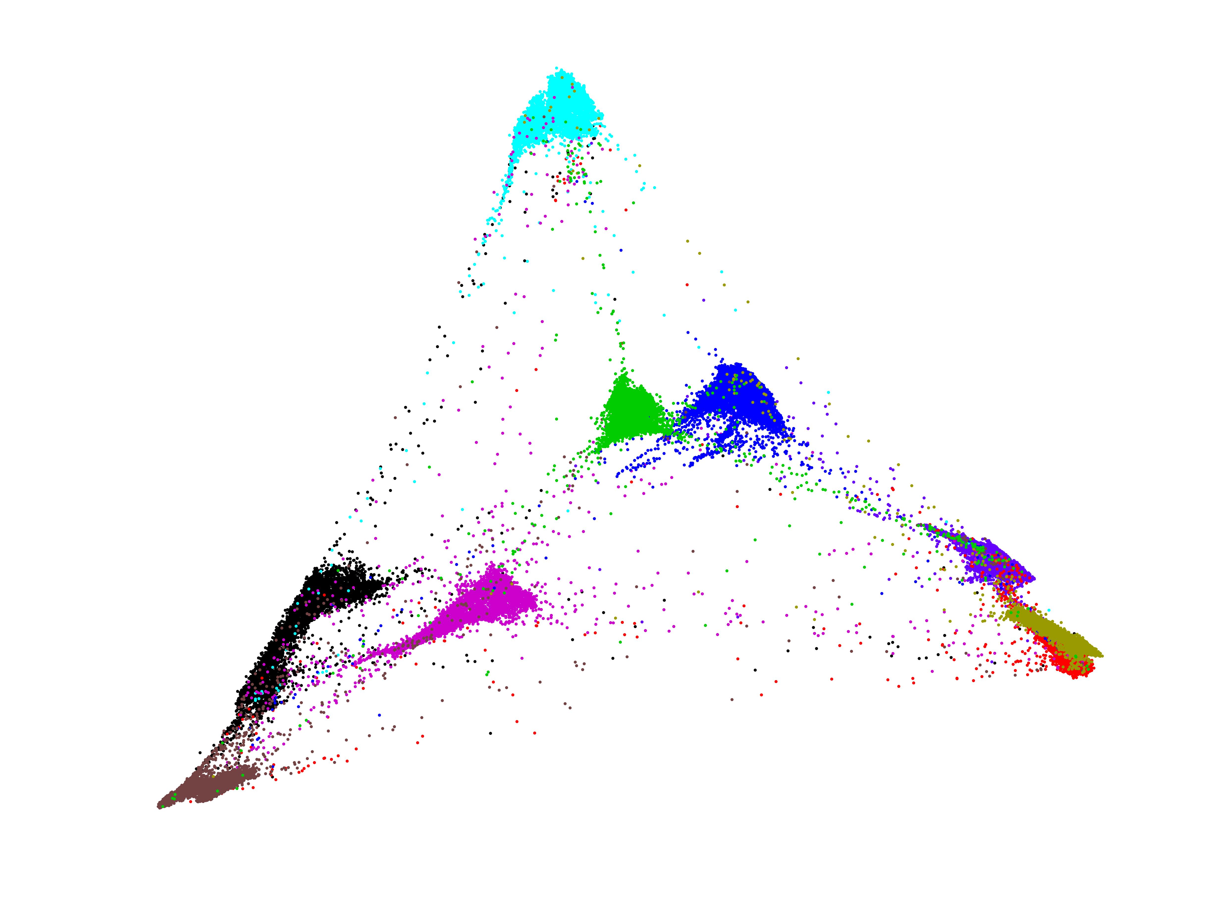
The above feature was produced under the default parameter setting of MBN, which can be downloaded here: MNIST_10dim. When used for clustering, it results in a clustering accuracy of 96.64% by both k-means and agglomerative hierarchical clustering.The original MNIST can be found at http://yann.lecun.com/exdb/mnist/.
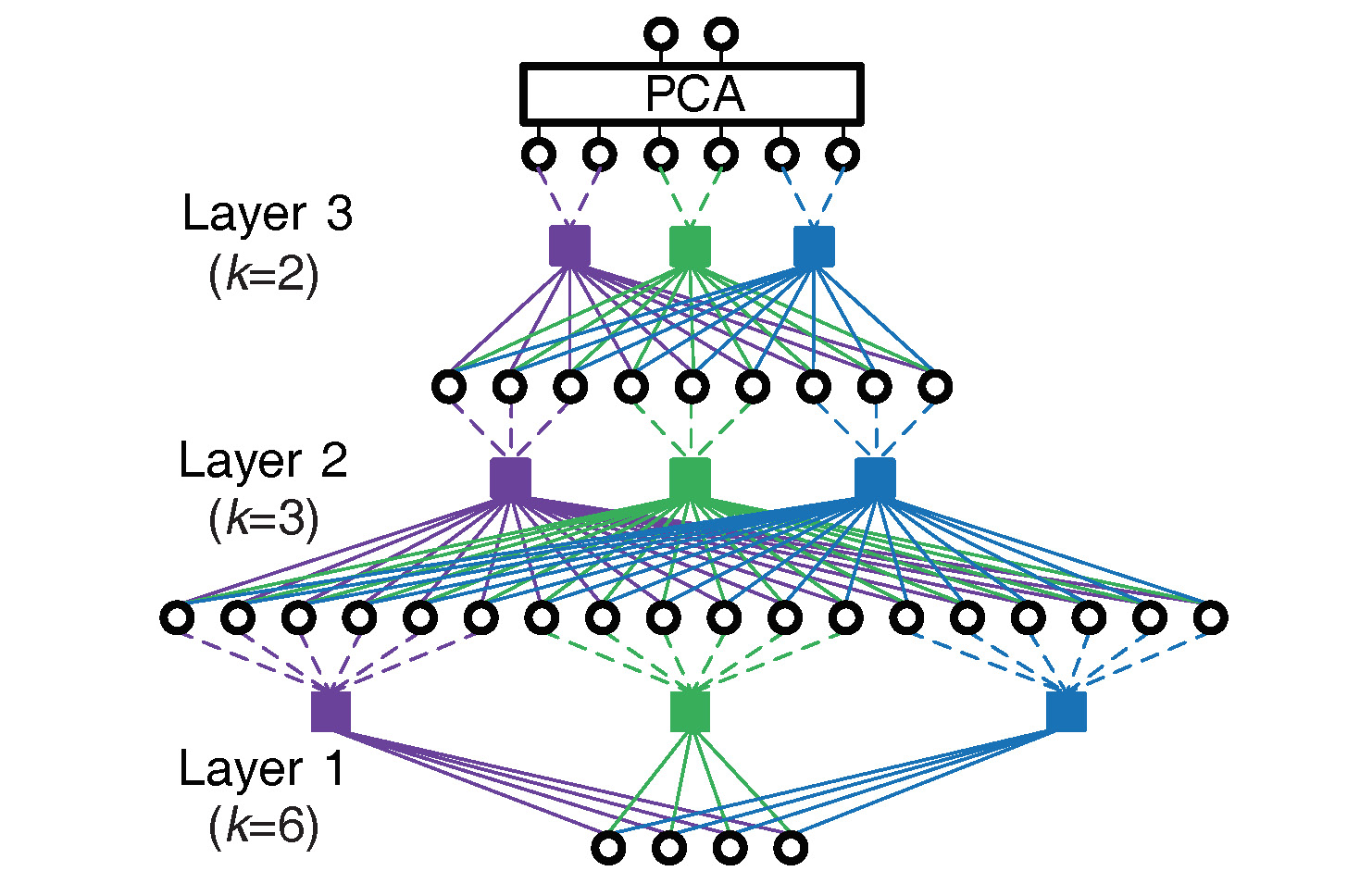
Given a dataset Z, MBN builds a multilayer network with L hidden layers from bottom-up, each layer contains V independent clusterings.
for LayerID = 1,2,...,L
{
for ClusteringID = 1,2,...,V
{
Step 1: Random resampling of feature (optional): Randomly sample a number of variables of Z to form a new set X
Step 2: Random resampling of data: Randomly sample k data points from X;
Step 3: One-nearest-neighbor learning: Take the k data points as the centers of a clustering model, and use the model to partition X into k disjoint clusters by one-nearest-neighbor learning. The clustering model outputs a one-hot representation for each datapoint in Z.
}
Step 4: Concatenate the one-hot representations produced by all clusterings into a sparse representation, and use the sparse representation as the input dataset of its upper layer, i.e. Z.
}
Note:
1) A key parameter setting: Parameter k from the bottom layer to the top layer should become smaller and smaller.
2) Post-processing: MBN may use any linear dimensionality reduction algorithm as the output layer to reduce the sparse representation to an explicit low-dimensional feature. Here we prefer principal component analysis (PCA).
MBN has the following properties:
1. Simple:
It contains only three simple operators--- random resampling, stacking, and one-nearest-neighbor optimization.
2. Effective:
It does not make model or prior assumptions of data.
It supports not ony large-scale data but also very small-scale data that contain only dozens of data points.
It does not suffer from outliers.
It does not suffer from bad local minima, though it is a multilayer nonlinear method.
It can be built as 'deep' as needed easily, where the word 'deep' refers to deep learning.
It produces good performance in a number of evaluated benchmark datasets without hyperparameter tunning. If the hyperparameters were tuned carefully, it produces better performance.
3. Efficient:
It supports parallel computing naturally.
Its time complexity grows linearly with the size of data.
Only the bottom layer costs some time, while other layers are computed efficiently.
MBN contains two core components---(1) each layer is a histogram-based density estimator which transforms the data space to a uniformly distributed probability space, and (2) a stack of such density estimators build a hierarchical structure which reduces the small principal components gradually by building a vast number of hierarchical trees implicitly.
1. Histogram-based density estimator
a) How strong is its representation ability?
The representation ability of a learning model can be understood as how fineness the model patitions the data space. A single-layer MBN can partition the data space to O(k*2^V) disconnected fractions, while a single-layer binary neural network with V hidden units can partition the data space to O(2^V) disconnected fractions [2]. Hence, the representation ability of MBN is linearly larger than that of a binary neural network.
b) Why does the simple random resampling build an effective density estimator?
c) Why use binarization by one-nearest-neighbor learning?
MBN estimates the (frequentist) probabilistic similarity of any two data points by the number of the cluster centers they share in common over V votes, which is a histogram-based density estimator. After binarization, we do not need probability model assumptions anymore, such as Gaussian assumption. As we know, model assumptions cause many unwanted problems.
d) Do we lose much information from the binarization?
The density estimator does not lose much information. As presented in item 1.a, the representation ability is determined by how subtle the data space can be partitioned. We have proved that the loss is linearly decreased to a small value by increasing the number of the base clusterings, which is similar to the proof of the generalization of random forests [4].
2. Hierarchical structure
a) Why hierarchical structure?
The histogram-based density estimator encodes most information into the probability space, including unwanted noise, nonlinearity, and small variances. Therefore, we need to further reduce the useless information. Deep learning provides the motivation, where the upper layers compress the input into abstract representations. Here we emphasize that MBN is not a neural network, since it does not rely on backpropagation. We would prefer MBN an ensemble learning method since its theoretical foundation is built on ensemble learning.
b) How does the hierarchical structure work?
Suppose the parameters k from the bottom layer to the top layer are k1, k2,...,kt, with k1>k2>...>kt. Then, according to item 1.a, the number of the disconnected fractions from bottom-up are O(k1*2^V), O(k2*2^V),...,O(kt*2^V) respectively. It is obvious that O(k1*2^V)>O(k2*2^V)>...>O(kt*2^V), which means that the small fractions at the bottom layer, named leaf nodes, are gradually merged, to small fractions at the top layer, named root nodes. Because each root node corresponds to a tree, we see that MBN builds as many as O(kt*2^V) trees.
c) Will the hierarchical structure lose much information?
It depends on how the information is defined. We give two examples. If our purpose is for classification, e.g. clustering or content-based retrieval, we only need to get the classification labels, while all other information can be discarded as noise. From this point of view, MBN does not lose much information. However, if our purpose is for nearest-neighbor-search, such as instance-based retrieval, then MBN may slightly contaminate the accurate nearest-neighbor-chain (or called ranking order) of the data in the original space. For the latter, we may consider building a single layer network instead of a multilayer network.
d) What is the connection between MBN and random forests, given that both of them build trees?
First, MBN builds a vast number of trees on data space instead of on data points, while random forests build a handful trees on data points directly. It is easy to see that the data space around a data point may be partitioned to many disconnected fractions by MBN. Second, MBN uses the root nodes of trees as the representation of data, while each tree of random forests uses its leaf nodes to select a nearest neighbor of a given test data point for voting in the original data space. Hence, their trees are fundamentally different.
* One comment on the name of MBN
The keyword bootstrap refers to a data resampling method, named bootstrap resampling [5], which resamples data with replacement. When MBN trains a number of k-centroids clustering at each layer, it samples data with replacement where the sample is used as the centroids. Therefore, there may be some common centroids between two k-cetroids clusterings, which causes correlation between the clusterings. To decorrelate the k-centroids clusterings, the random selection of features are adopted.
If we take a look at the training of each single k-centroids clustering, MBN resamples data without replacement which is another method---delete-d jackknife resampling [6].
We ran MBN with the default setting. For comparison, we took PCA, spectral clustering [7], and t-SNE [8] as the baselines. When running spectral clustering with non-text data, we use Gaussian kernel with the kernel width determined automatically by the average Euclidean distance between data points. We apply the low-dimensional output to k-means clustering. We also list the MBN with the agglomerative hierarchical clustering.
We evaluated the comparison methods in terms of discriminant trace (DT) criterion [9][10, eq. (4.50)], clustering accuracy (ACC) , and normalized mutual information (NMI) [11], where the DT criterion directly evaluates the discriminant ability of the learned features by measuring the between-class variances over within-class variances. The larger the DT score is, the better the comparison method behaves.
We ran the comparison on the following four representative datasets for 10 times and reported the average performance. The average results are listed in the follow tables. The statistical significance is evaluated by the two tailed-t test whose null hypothesis is at the 5% significance level. The datasets and overall results of the 10 independent runs have been incorporated in the MATLAB toolbox of MBN.
1. MNIST5000
This data set contains 5000 random selected images belonging to 10 handwritten digits from MNIST
| DT score | ACC | NMI | |
| MBN | 6.36 | 82.5% | 0.776 |
| PCA | 0.26 | 52.7% | 0.498 |
| Spectral clustering | 0.80 | 52.0% | 0.476 |
| t-SNE | 4.67 | 72.8% | 0.695 |
| *MBN with hierarchical clustering | 6.37 | 81.6% | 0.773 |
2. Speaker recognition
This data set contains 4000 utterances belonging to 200 speakers. This dataset is extracted from the training data of NIST SRE 2018 by the x-vector front-end.
| DT score | ACC | NMI | |
| MBN | 51.43 | 78.6% | 0.930 |
| PCA | 5.13 | 47.4% | 0.760 |
| Spectral clustering | 3.03 | 79.3% | 0.927 |
| t-SNE | 12.38 | 65.5% | 0.871 |
| *MBN with hierarchical clustering | 52.49 | 87.1% | 0.925 |
3. COIL-100
This data set contains 7200 images belonging to 100 objects.
| DT score | ACC | NMI | |
| MBN | 18.95 | 66.6% | 0.856 |
| PCA | 1.76 | 51.1% | 0.776 |
| Spectral clustering | 3.33 | 52.6% | 0.779 |
| t-SNE | 10.27 | 60.5% | 0.829 |
| *MBN with hierarchical clustering | 18.66 | 68.8% | 0.862 |
4. 20-Newsgroups
This text corpus contains 18846 documents belonging to 20 classes.
| DT score | ACC | NMI | |
| MBN | 1.62 | 64.4% | 0.536 |
| PCA | 0.52 | 41.6% | 0.466 |
| Spectral clustering | 1.06 | 46.4% | 0.506 |
| t-SNE | 3.66 | 64.4% | 0.597 |
| *MBN with hierarchical clustering | 1.63 | 60.4% | 0.536 |
1. Code
MBN code with demos: MBN_toolbox_v7.rar [25MB] (Note: You need MATLAB R2017a and after to run the t-SNE baseline as a built-in function of MATLAB.)
2. Key functions
It takes PCA as a preprocessing stage, which reduces the data to no more than 100 dimensions for the computational efficiency.
It supports the standard PCA, linear kernel based sparse kernel PCA (recommended) [12], EM-PCA [13], spectral clustering, or tsne-MBN as the output layer, where tsne-MBN is a revised t-SNE that constructs the density affinity matrix of data by the output of the top hidden layer of MBN instead of the original affinity matrix construction method of t-SNE.
It supports k-means clustering or agglomerative hierarchical clustering as the clustering tool. When the number of classes is unknown, then agglomerative hierarchical clustering determines the number of classes on-the-fly.
3. Parameters
The MATLAB MBN function is MBN(data, c, param), where
| Parameter name | Description | Default value |
| ktop | Parameter k of the k-centroids
clustering at the top layer. It should be set to guarantee that at
least one data point per class is selected in each random sample,
which guarantees that the random resampling is still stronger than
random guess. Note: 'ktop' is important. When 'c' is not given or when the data is severely class-imbalanced, user should better set 'ktop' manually. |
1.5c, when parameter 'c' is given; 100, when parameter 'c' is not given |
| k1 | Parameter k of the k-centroids clustering at the bottom layer. | min(0.5N, 10000) |
| delta | delta = k(t)/k(t-1), where k(t-1) and k(t) represent the parameters k at two adjacent layers. It is a value between 0 and 1 | 0.5 |
| a | Ratio of randomly sampled dimensions over D. It is a value betwen 0 and 1. | 0.5 |
| V | Number of k-centroids clustering per layer. | 400 |
| k | Parameter k of the k-centroids clustering at all layers. It is determined jointly by 'ktop', 'k1' and 'delta'. However, users may specify 'k' as a vector, such as [100,80,50], which defines an MBN of three layers. If 'k' is set, then 'ktop', 'k1' and 'delta' are disabled. | |
| s | Similarity measurement at the bottom layer. It can be set to 'e' and 'l'. 'e' means Euclidean distance. 'l' means inner-product similarity. | 'e' |
| m | Determine whether the MBN model will be saved for prediction. It can be set to 'yes' or 'no'. Because we do not provide MBN_predict function any more in new software versions. Users may always set it to 'no'. | 'no' |
| f | Determine whether the sparse feature at each hidden layer will be saved. It can be set to 'yes' or 'no'. | 'no' |
| d | Number of the dimensions of the MBN output. It is valied when the output layer is PCA or spectral clustering only. | c |
| ifPCA | Determine whether the input data is preprocessed by PCA. It can be set to 'yes' or 'no'. | 'yes' |
| inputdim | Determine the maximum number of dimensions of the input data after the PCA preprocessing. | 100 |
| ifCluster | Determine whether using the low-dimensional output of MBN for clustering. It can be set to 'yes' or 'no'. | 'yes' |
| ClusterTool | Determine which clustering algorithm is used. It can be set to 'kmeans' and 'ahc'. 'kmeans' is the k-means clustering algorithm. 'ahc' is the agglomerative hierarchical clustering. | 'kmeans' |
| outputlayer | Determine which kind of output layer is adopted. It
can be set to 'pca', 'spca', 'empca', 'spectral', and 'tsne-mbn'. 'pca'
is the built-in PCA function of MATLAB. 'spca' is the linear kernel
based kernel PCA. 'empca' is the expectation-maximization PCA
(EM-PCA). 'spectral' is the Laplacian matrix decomposition of the
linear kernel based the spectral clustering. 'tsne-mbn' is an MBN
revised t-SNE
nonlinear dimensionality reduction method that uses the output of
MBN to construct the affinity matrix of t-SNE.
If the data set is larger than 10000 data points, 'spca' takes at most 10000 data points to do eigenvalue decomposition of the linear kernel matrix. Users may change this limitation in the MBN function. |
'spca' |
| nWorkers | Determine how many workers will be used for the parallel computing. | maximum number of physical cores of CPU |
4. Examples
Although we have defined many parameters, we use their default values at most of the time. Here we list some usages for users' reference:
| Situations | Solutions | Example functions |
| Class-balanced data | Default setting | MBN(data, c) |
| Class-imbalanced data | Need to specify parameter 'ktop'. See the description of 'ktop'. | MBN(data, c, {'ktop', 300}) |
| Number of classes unknown | Need to specify parameter 'ktop'. If 'ktop' is not given explictly, then MBN will use the default value 'ktop' = 100. | MBN(data, [], {'ktop', 50}) |
| Need to build a deeper model than the default | Set 'delta' larger than the default, i.e. 0.5. | MBN(data, c, {'delta', 0.8}) |
| Need to control the memory occupacy. | Set 'k1' to a limited number, which may sacrifice performance. | MBN(data, c, {'k1', 2000}) |
| Need to denoise data that have simple distributions. | Set MBN to a single layer | MBN(data, c, {'k1', 50, 'delta', 0}) |
| Need to use original data as input | Disable the PCA preprocessing, with the risk of high computational cost. | MBN(data, c, {'ifPCA', 'no'}) |
| Text data (or similar very high-dimensional sparse data) | The most common similarity measurement for text data is cosine similarity, therefore, we should first normalize data and then use inner-product as the similarity measure of the bottom layer. Because text data is very sparse, we should set 'a' = 1 to prevent information loss in the inner-product operator. | MBN(data, c, {'s', 'l', 'a', 1, 'ifPCA', 'no'}) |